IMU Sensors in Sport: Why Understanding Quaternions Is Non-Negotiable

A few months ago I was working on a sensor for velocity-based training: a device that clips onto a barbell and tells a coach how fast the athlete is moving the bar. Sounds simple. You put an accelerometer on the bar, read the acceleration, integrate it to get velocity.

Then the problem hits you in about five minutes of testing: the barbell rotates. During a squat, a deadlift, a press, the bar never stays perfectly level. It tips forward, it rolls slightly in the hands, it bends under load. And when it does, the sensor rotates with it.

The axis the sensor is measuring is no longer the axis you care about.

---

Step back: why measure acceleration at all?

Velocity is the integral of acceleration. If you know how fast something is accelerating at every instant and add those values up over time, you get its velocity.

Accelerometers are cheap, small, and accurate. A combined IMU chip with both accelerometer and gyroscope costs a few euros and fits on a fingernail. You strap it to the barbell, sample it 100 times per second, and integrate.

But integrate what, exactly? The acceleration in which direction?

For a barbell exercise, we care about one thing: vertical velocity. The bar goes up and down. Gravity pulls in one direction. The athlete pushes against gravity. The number that tells you whether the athlete is fast or fatigued is how fast the bar moves vertically, relative to the floor.

So the question is: how do you know which direction is vertical?

---

The problem: two axes that don’t agree

When the sensor is bolted perfectly flat to the bar, its Z axis points straight up. Reading Z gives you vertical acceleration. Easy.

But clip a sensor to a real barbell and it will never sit perfectly flat. Mount it slightly off, drop it, swap it between sessions, and the alignment changes. Worse: even if you start perfectly aligned, the bar moves during the lift. A barbell that rotates 20 degrees has just shifted which axis its sensor is measuring.

The sensor has its own coordinate frame: X, Y, Z fixed to its body. The world has its own coordinate frame: X, Y, Z fixed to the room, with Z always pointing up toward the ceiling. When the sensor tilts, its Z axis points somewhere diagonal in space, not up, not sideways, somewhere in between. And the acceleration it reports on Z is a mixture of all three world directions.

If you integrate that number, you get velocity in the wrong direction. You might read the barbell as moving sideways when it is moving up. You might miss vertical motion entirely because the sensor is perpendicular to gravity.

---

The fix: quaternions and the Madgwick filter

The obvious approach: track the sensor’s rotation using pitch, roll, and yaw — the three angles that describe how it is oriented in space. Then reverse the rotation mathematically to recover the world-frame acceleration.

This works, until the sensor reaches an orientation where pitch is exactly 90 degrees. At that point, pitch and yaw become the same axis. Rotating around one is geometrically identical to rotating around the other. You have lost a degree of freedom. The math breaks down.

This is gimbal lock, and it is not a software bug. It is a mathematical singularity that cannot be patched. For a barbell sensor that might tip sideways during a heavy deadlift or an overhead press, it is a real concern.

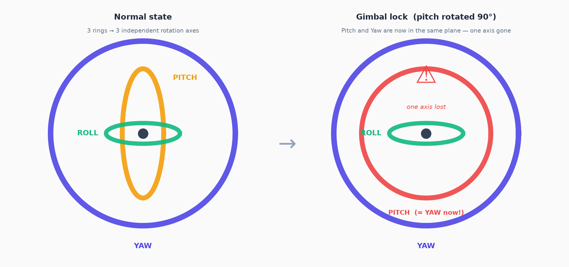
The solution is to represent orientation with quaternions instead of Euler angles.

A quaternion is four numbers that encode a rotation as one angle around one axis. Unlike Euler angles, there is no combination of orientations that collapses two axes into one. Gimbal lock simply cannot happen.

But knowing the rotation format is not enough. You also need to estimate, at every moment, how the sensor is actually oriented. That is the job of the Madgwick filter: it fuses the gyroscope and the accelerometer to produce a fresh orientation estimate every 10 ms, tracking how the sensor moves in real time.

The filter produces a quaternion. You apply the quaternion to the raw sensor reading. You get the correct vertical acceleration. You integrate. You have velocity.

---

For the mathematically curious

Not interested in the equations? Skip to The logic in plain English — the diagram below explains the whole approach without formulas.

Quaternions

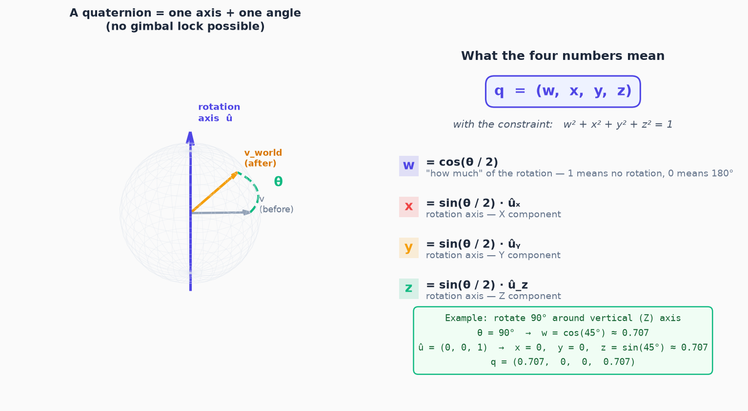
A quaternion is four numbers: (w, x, y, z). They always satisfy one rule:

w² + x² + y² + z² = 1

That constraint keeps the quaternion on the surface of a four-dimensional unit sphere. Think of it like a point on a globe, but one dimension higher.

The four numbers encode a rotation as one angle around one axis:

• w = cos(θ/2) — the cosine of half the rotation angle
• (x, y, z) = sin(θ/2) · û — the rotation axis scaled by the sine of half the angle

A 90° rotation around the vertical Z axis gives θ = 90°, so w = cos(45°) ≈ 0.707, z = sin(45°) ≈ 0.707, x = y = 0. One quaternion, one unambiguous rotation.

To rotate a vector v from the sensor frame to the world frame:

v_world = q · v · q⁻¹

Where q⁻¹ is the conjugate of the quaternion (flip the sign of x, y, z). This expands to the three dot-product lines in the code below.

The Madgwick filter

The gyroscope and accelerometer fail in opposite ways.

The gyroscope tracks fast rotations accurately and is immune to vibration. But it drifts. Its small constant error accumulates into a steadily growing offset that has nothing to do with reality. Leave it running for a few minutes and the orientation estimate is noticeably wrong, even if the sensor barely moved.

The accelerometer always knows where gravity is. When the sensor is still, it gives an absolute reference for which way is up. During motion, it also picks up the bar’s own acceleration and becomes noisy. But at every moment of stillness — between reps, at the bottom of a lift — it provides a correction.

The filter combines both in three steps every 10 ms.

Step 1 — gyroscope prediction. The gyroscope reading (gx, gy, gz) is treated as a pure quaternion ω = (0, gx, gy, gz) and used to predict how the orientation changed since the last sample:

q̇_gyro = ½ × q ⊗ ω

Where ⊗ is quaternion multiplication and q is the current orientation estimate. Fast and precise, but accumulates drift.

Step 2 — accelerometer correction. The accelerometer reading is normalised to a unit vector â. If q were perfect, rotating the world gravity vector (0, 0, 1) by q⁻¹ should give exactly â. The difference is the error. The filter computes the gradient of that error with respect to q — the direction in quaternion space that reduces the mismatch most rapidly:

q̇_∇ = ∇f(q, â)

Accurate, but noisy during motion, so it is applied gently.

Step 3 — blend and integrate. β controls how much weight goes to the correction:

q_{t+1} = q_t + ( q̇_gyro − β × q̇_∇ ) × Δt

The filter then normalises the result to keep q on the unit sphere.

Dynamic β

A fixed β works, but a smarter approach adjusts it every step based on what the accelerometer is actually seeing.

When the sensor is still, the accelerometer reads exactly 1g: pure gravity, reliable correction. Raise β to fix drift faster.

When the bar is moving fast, the accelerometer also picks up the bar’s inertia. Its reading departs from 9.81 m/s². The correction becomes misleading. Lower β, trust the gyroscope more.

A practical implementation:

float a_mag = sqrtf(ax*ax + ay*ay + az*az);
float deviation = fabsf(a_mag - 9.81f) / 9.81f;  // 0 = perfect 1g, 1 = completely off

// Smooth interpolation: high beta when still, low beta when moving
float beta = 0.01f + (0.08f - 0.01f) * expf(-6.0f * deviation);

At rest (deviation ≈ 0), β ≈ 0.08: drift corrects quickly. Mid-lift (deviation ≈ 0.4), β ≈ 0.02: the gyroscope dominates and the lift trajectory stays clean. The filter tunes itself.

---

The logic in plain English

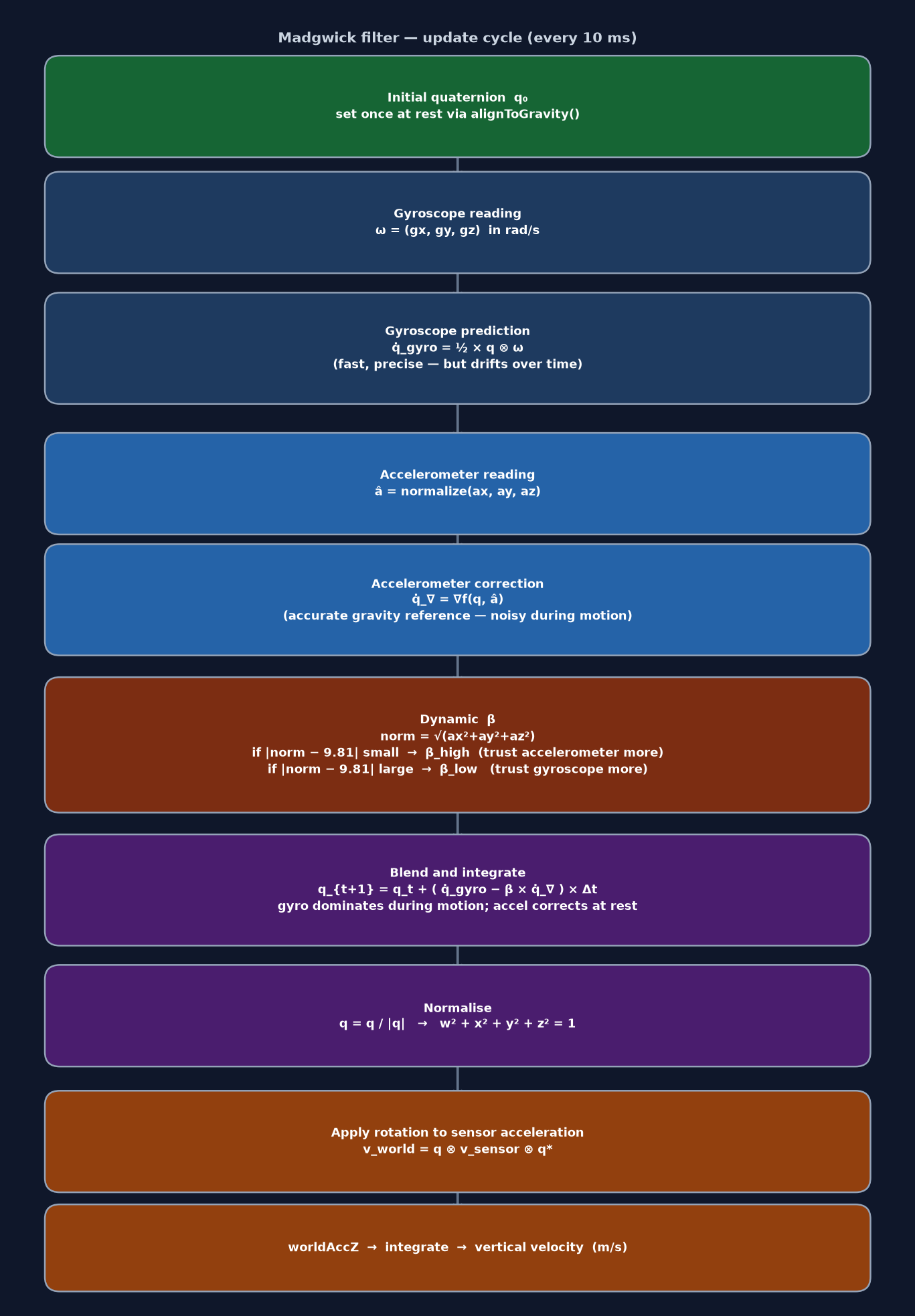
The diagram below shows the full update cycle. No notation required.

What a quaternion actually is. Four numbers that describe exactly how the sensor is rotated in space — one angle around one axis. Where Euler angles break down when two axes collapse into one (gimbal lock), quaternions never do. The image in the math section above shows this geometrically, but you do not need to follow the algebra to use the result. The filter gives you the quaternion; you apply it to the sensor data.

How the filter works. Two inputs compete to steer the orientation estimate at every step.

The gyroscope tells the filter how the sensor rotated since the last sample. Trusted alone, it would track rotation precisely — but it has a tiny constant error that accumulates into visible drift over minutes.

The accelerometer provides a reference against that drift. It always knows where gravity is. When the sensor is still, that reference is clean and reliable. When the sensor is moving fast, it also picks up the bar’s inertia and becomes unreliable.

β decides who wins. And dynamic β makes that decision automatically, every 10 milliseconds, by checking how close the accelerometer’s reading is to 1g. Close: trust the accel correction. Far: trust the gyro instead.

The output is a fresh quaternion every 10 ms. Apply it to the sensor’s acceleration reading and you always get the correct world-frame vector, regardless of how the barbell is oriented.

---

What the data shows

The clearest way to see the problem is to integrate both versions — raw sensor-frame and quaternion-corrected — into velocity and compare:

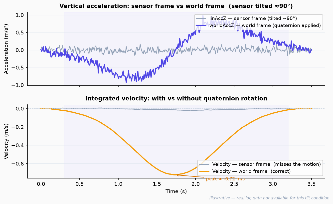
The sensor in this test was mounted at a significant angle, roughly 120 degrees off vertical. The grey curve barely moves because the sensor’s Z axis was pointing nearly sideways: it was measuring a projection of vertical acceleration close to zero, so integrating it gives close to zero velocity regardless of how fast the bar moved. The amber curve correctly tracks the bar descending at up to 1.3 m/s — the same motion, seen through the quaternion rotation that realigns Z to the true vertical.

The bar moved. The sensor did not know it.

For a complete rep, here is what the correctly oriented signal looks like — velocity on the left, acceleration on the right:

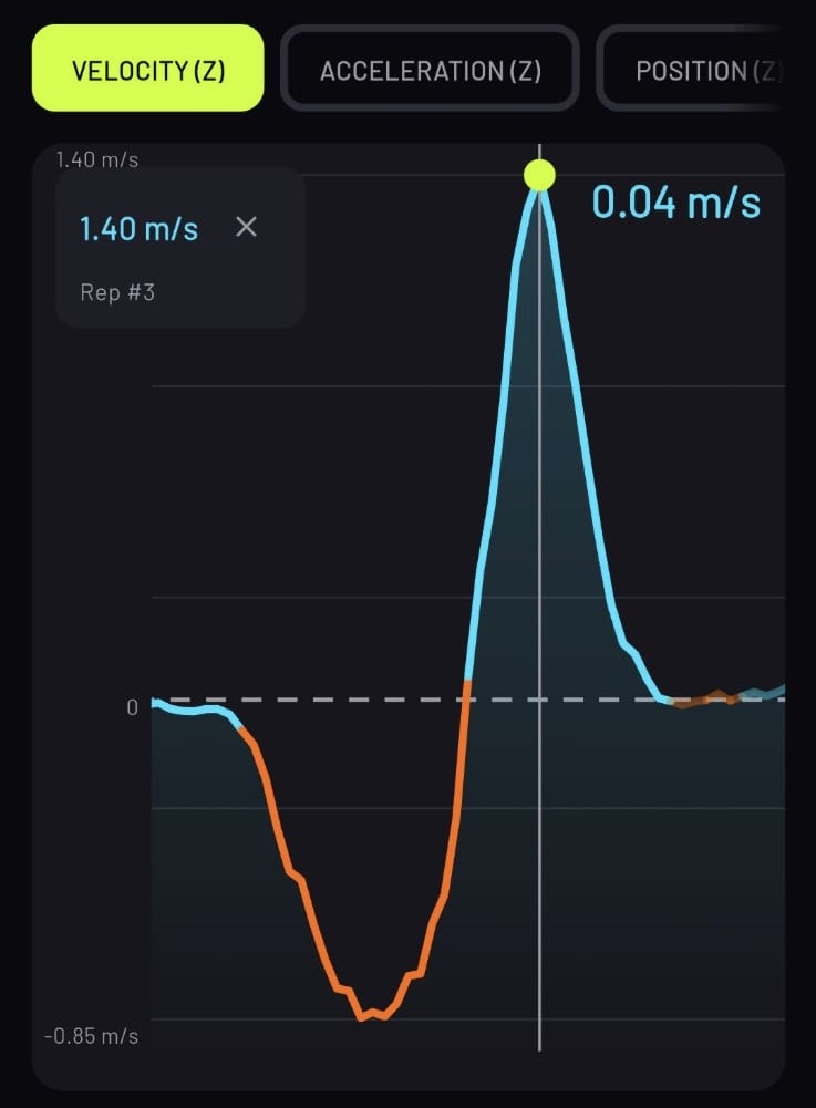
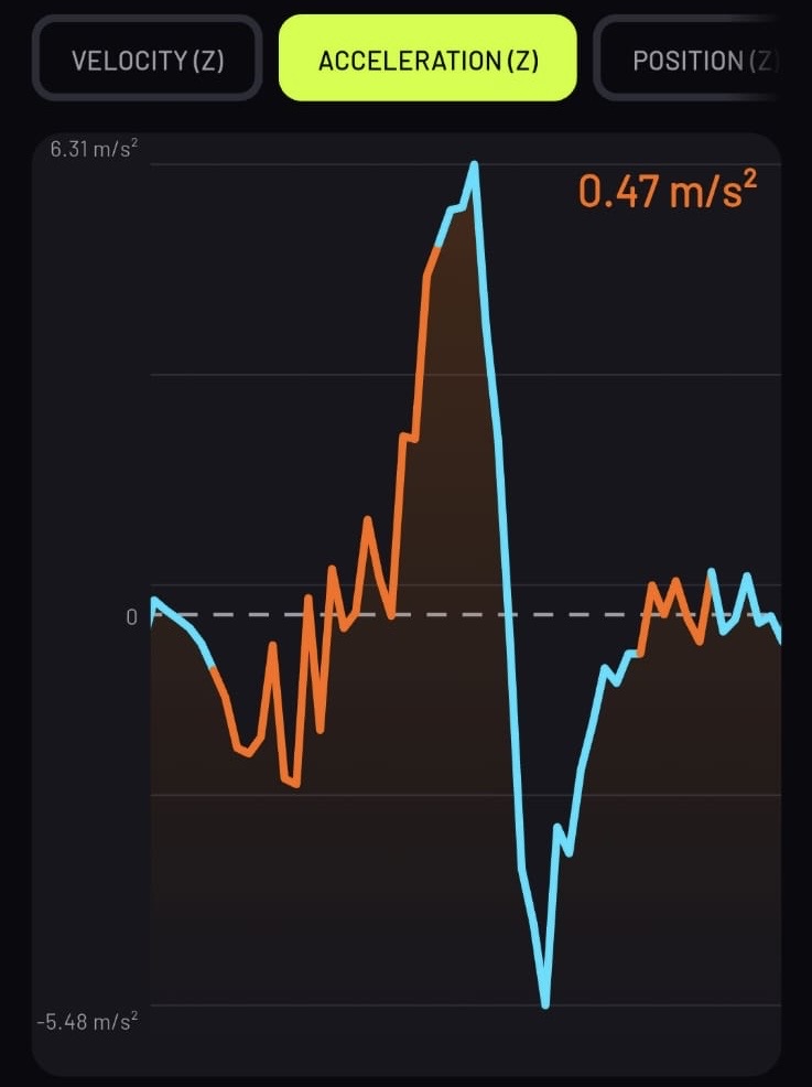
The velocity starts at zero, drops negative as the athlete lowers the bar (eccentric, orange), then climbs sharply positive as the athlete drives it back up (concentric, cyan). The concentric peak of +1.40 m/s is the number a coach uses to monitor bar speed and infer fatigue. The asymmetry is worth noticing: the eccentric descent is broad and rounded, the concentric ascent is a narrow spike. The athlete is braking on the way down and exploding on the way up.

The acceleration tells the same story, but noisier. The oscillation during the eccentric is real — the athlete is fighting inertia and adjusting continuously. The sharp spikes at the transition are the impulse of the drive followed by the deceleration at lockout. Without the quaternion rotation, both curves would be nearly flat regardless of how fast the bar moved.

---

The code, step by step

A minimal Arduino sketch that implements this. Every line is commented:

#include "MadgwickAHRS.h"  // the filter library

MadgwickAHRS filter;  // one filter instance for the whole session

void setup() {
  imu.begin();              // start the IMU
  filter.reset();           // set quaternion to identity (no rotation assumed)

  // Read the accelerometer while the sensor is perfectly still.
  // This aligns the filter's reference frame to gravity — so the world
  // frame is correct from the very first rep.
  float ax, ay, az;
  imu.readAccel(ax, ay, az);
  filter.alignToGravity(ax, ay, az);
}

void loop() {
  float gx, gy, gz;   // angular velocity in degrees/s (from gyroscope)
  float ax, ay, az;   // raw acceleration in m/s² (from accelerometer)
  imu.readGyro(gx, gy, gz);
  imu.readAccel(ax, ay, az);

  float dt = 0.01f;  // 10 ms between samples — 100 Hz

  // --- Madgwick filter update ---
  // Dynamic beta: trust the accelerometer more when the sensor is still (norm ≈ 1g),
  // trust the gyroscope more when the bar is moving fast (norm departs from 1g).
  float a_mag   = sqrtf(ax*ax + ay*ay + az*az);
  float deviation = fabsf(a_mag - 9.81f) / 9.81f;
  float beta    = 0.01f + 0.07f * expf(-6.0f * deviation);

  // Runs three steps internally: gyroscope prediction (q̇_gyro = ½ q ⊗ ω),
  // accelerometer correction (q̇_∇ = ∇f(q, â)), and blend (q += (q̇_gyro − β·q̇_∇)·Δt).
  // After this call, filter.q0–q3 describe how the sensor is oriented right now.
  filter.update(gx, gy, gz, ax, ay, az, dt, beta);

  // --- Rotate acceleration from sensor frame to world frame ---
  float q0 = filter.q0(), q1 = filter.q1(),
        q2 = filter.q2(), q3 = filter.q3();

  // Subtract gravity from the sensor reading (gravity = 9.81 m/s² along sensor Z)
  float linAccX = ax;
  float linAccY = ay;
  float linAccZ = az - 9.81f;  // remove the 1g contribution before rotating

  // Apply the quaternion rotation — sensor frame → world frame.
  // These three lines are the core of the whole approach.
  float worldAccX = (1 - 2*(q2*q2 + q3*q3)) * linAccX
                  + (2*(q1*q2 - q0*q3))      * linAccY
                  + (2*(q1*q3 + q0*q2))      * linAccZ;

  float worldAccZ = (2*(q1*q3 - q0*q2))      * linAccX
                  + (2*(q2*q3 + q0*q1))      * linAccY
                  + (1 - 2*(q1*q1 + q2*q2))  * linAccZ;

  // worldAccZ is now the true vertical acceleration in m/s²,
  // regardless of how the barbell is oriented.

  // --- Integrate acceleration to get vertical velocity ---
  // Trapezoidal rule: average the current and previous sample, multiply by time step.
  static float velZ = 0;
  static float prevAcc = 0;
  velZ += (worldAccZ + prevAcc) * 0.5f * dt;  // velocity accumulates each sample
  prevAcc = worldAccZ;

  // velZ is now vertical velocity in m/s.
  // Positive = moving up, negative = moving down.
}

The rotation is three dot products — one per output axis. You feed in the sensor-frame vector, you get out the world-frame vector. The filter abstracts the quaternion update; the rotation formula never changes regardless of orientation.

---

Why this matters in practice

The problem is not exotic. Any time you mount a sensor on something that rotates — and every barbell rotates — reading the sensor’s Z axis raw gives you the wrong number. The error scales with the tilt angle: 10 degrees off and you are 2% wrong, 30 degrees and you are 13% wrong, 90 degrees and you are measuring something completely orthogonal to what you intended.

Velocity-based training makes decisions based on small differences. A drop from 1.0 to 0.85 m/s might be the threshold for stopping a set. If the measurement itself is off by 10–15% depending on how the sensor happens to be sitting, those thresholds are meaningless.

The quaternion rotation fixes this. The Madgwick filter estimates the orientation continuously so the rotation is always current, even as the bar moves. The cost is a few microseconds of computation per sample and a filter parameter you tune once.

The sensor does not need to know which way is up. The filter figures it out.